Before Getting Started make sure you got pip and python 3.8 or higher
I am using a Jupyter Notebook and I might already have these libraries but going to run it just in case
1
| pip install pandas numpy matplotlib yfinance seaborn
|
These are the following companies we are going to use for analyzing:
San Miguel Corporation (SMGBF)
Jollibee Foods Corporation (JBFCY)
Universal Robina Corporation (UVRBF)
Mondelez International, Inc.(MDLZ)
yfinance is a library for fetching historical stock data
pandas for Data Exploration and Data Cleaning
seaborn and matplotlib for Data Visualization (Honestly when I heard about these in 2016 or 17 I thought these were YouTubers)
1
2
3
4
| #pandas and NumPy imports
import pandas as pd
from pandas import Series,DataFrame
import numpy as np
|
1
2
3
4
5
| # For Visualization
import matplotlib.pyplot as plt
import seaborn as sns
sns.set_style('whitegrid')
%matplotlib inline
|
1
2
3
4
| import os #for files read/write
from datetime import datetime # For time stamps
import yfinance as yf #fetching the data stock
from __future__ import division# For division in Python 3
|
1
2
3
4
5
6
7
8
| # Fetch stock data
def fetch_stock_data(ticker, start_date, end_date):
stock_data = yf.download(ticker, start=start_date, end=end_date)
return stock_data
smg_data = fetch_stock_data('SMGBF', '2021-01-01', '2023-12-31')
jbf_data = fetch_stock_data('JBFCY', '2021-01-01', '2023-12-31')
uvr_data = fetch_stock_data('UVRBF', '2021-01-01', '2023-12-31')
delm_data = fetch_stock_data('MDLZ', '2021-01-01', '2023-12-31')
|
[*********************100%***********************]  1 of 1 completed
[*********************100%***********************]  1 of 1 completed
[*********************100%***********************]  1 of 1 completed
[*********************100%***********************]  1 of 1 completed
checking data
1
2
3
4
| print(smg_data.head())
print(jbf_data.head())
print(uvr_data.head())
print(delm_data.head())
|
Price          Close      High       Low      Open Volume
Ticker         SMGBF     SMGBF     SMGBF     SMGBF  SMGBF
Date
2021-01-04  2.550820  2.550820  2.550820  2.550820      0
2021-01-05  2.479167  2.479167  2.479167  2.479167   1100
2021-01-06  2.479167  2.479167  2.479167  2.479167      0
2021-01-07  2.479167  2.479167  2.479167  2.479167      0
2021-01-08  2.479167  2.479167  2.479167  2.479167      0
Price           Close       High        Low       Open Volume
Ticker          JBFCY      JBFCY      JBFCY      JBFCY  JBFCY
Date
2021-01-04  15.941961  15.941961  15.941961  15.941961    500
2021-01-05  15.941961  15.941961  15.941961  15.941961      0
2021-01-06  15.941961  15.941961  15.941961  15.941961      0
2021-01-07  14.946193  15.139546  14.946193  14.946193   1100
2021-01-08  14.946193  14.946193  14.946193  14.946193      0
Price          Close      High       Low      Open Volume
Ticker         UVRBF     UVRBF     UVRBF     UVRBF  UVRBF
Date
2021-01-04  2.765748  2.765748  2.765748  2.765748      0
2021-01-05  2.765748  2.765748  2.765748  2.765748      0
2021-01-06  2.765748  2.765748  2.765748  2.765748      0
2021-01-07  2.765748  2.765748  2.765748  2.765748      0
2021-01-08  2.844769  2.844769  2.844769  2.844769   5000
Price           Close       High        Low       Open   Volume
Ticker           MDLZ       MDLZ       MDLZ       MDLZ     MDLZ
Date
2021-01-04  52.686432  54.578488  52.149747  53.204931  9187200
2021-01-05  52.741009  52.868358  52.140646  52.659141  5421900
2021-01-06  52.640957  53.059395  52.449933  52.750116  7663200
2021-01-07  52.540890  53.077578  52.167937  52.504507  8589100
2021-01-08  52.932041  53.004814  52.149752  52.186135  6642700
checking for dupes
1
2
3
4
| print(smg_data.isnull().sum())
print(jbf_data.isnull().sum())
print(uvr_data.isnull().sum())
print(delm_data.isnull().sum())
|
1
| type(smg_data) #I just like to check what type of data we are working with
|
checking excel file
1
2
3
| path = 'fnbStocks.xlsx'
isExist = os.path.exists(path)
print(isExist)
|
True
So there was an error making the excel and here you would see that the columns for our data frame has two values
| Price | Close | High | Low | Open | Volume |
|---|
| Ticker | SMGBF | SMGBF | SMGBF | SMGBF | SMGBF |
|---|
| Date | | | | | |
|---|
| 2021-01-04 | 2.550820 | 2.550820 | 2.550820 | 2.550820 | 0 |
|---|
| 2021-01-05 | 2.479167 | 2.479167 | 2.479167 | 2.479167 | 1100 |
|---|
| 2021-01-06 | 2.479167 | 2.479167 | 2.479167 | 2.479167 | 0 |
|---|
| 2021-01-07 | 2.479167 | 2.479167 | 2.479167 | 2.479167 | 0 |
|---|
| 2021-01-08 | 2.479167 | 2.479167 | 2.479167 | 2.479167 | 0 |
|---|
| ... | ... | ... | ... | ... | ... |
|---|
| 2023-12-22 | 1.920405 | 1.920405 | 1.920405 | 1.920405 | 0 |
|---|
| 2023-12-26 | 1.920405 | 1.920405 | 1.920405 | 1.920405 | 0 |
|---|
| 2023-12-27 | 1.880809 | 1.969900 | 1.880809 | 1.969900 | 3000 |
|---|
| 2023-12-28 | 1.880809 | 1.880809 | 1.880809 | 1.880809 | 0 |
|---|
| 2023-12-29 | 1.880809 | 1.880809 | 1.880809 | 1.880809 | 0 |
|---|
753 rows × 5 columns
1
| display(smg_data.columns)
|
MultiIndex([( 'Close', 'SMGBF'),
            (  'High', 'SMGBF'),
            (   'Low', 'SMGBF'),
            (  'Open', 'SMGBF'),
            ('Volume', 'SMGBF')],
           names=['Price', 'Ticker'])
reassigned every dataframe with a new column
1
2
3
4
| smg_data.columns= [col[0] for col in smg_data.columns]
jbf_data.columns=[col[0] for col in jbf_data.columns]
uvr_data.columns=[col[0] for col in uvr_data.columns]
delm_data.columns=[col[0] for col in delm_data.columns]
|
1
| display(smg_data.columns)
|
Index(['Close', 'High', 'Low', 'Open', 'Volume'], dtype='object')
| Close | High | Low | Open | Volume |
|---|
| Date | | | | | |
|---|
| 2021-01-04 | 2.550820 | 2.550820 | 2.550820 | 2.550820 | 0 |
|---|
| 2021-01-05 | 2.479167 | 2.479167 | 2.479167 | 2.479167 | 1100 |
|---|
| 2021-01-06 | 2.479167 | 2.479167 | 2.479167 | 2.479167 | 0 |
|---|
| 2021-01-07 | 2.479167 | 2.479167 | 2.479167 | 2.479167 | 0 |
|---|
| 2021-01-08 | 2.479167 | 2.479167 | 2.479167 | 2.479167 | 0 |
|---|
| ... | ... | ... | ... | ... | ... |
|---|
| 2023-12-22 | 1.920405 | 1.920405 | 1.920405 | 1.920405 | 0 |
|---|
| 2023-12-26 | 1.920405 | 1.920405 | 1.920405 | 1.920405 | 0 |
|---|
| 2023-12-27 | 1.880809 | 1.969900 | 1.880809 | 1.969900 | 3000 |
|---|
| 2023-12-28 | 1.880809 | 1.880809 | 1.880809 | 1.880809 | 0 |
|---|
| 2023-12-29 | 1.880809 | 1.880809 | 1.880809 | 1.880809 | 0 |
|---|
753 rows × 5 columns
1
2
3
4
5
| with pd.ExcelWriter('fnbStocks.xlsx') as writer:
smg_data.to_excel(writer, sheet_name='SanMiguel')
jbf_data.to_excel(writer, sheet_name='Jollibee')
uvr_data.to_excel(writer, sheet_name='Robina')
delm_data.to_excel(writer, sheet_name='DelMonte')
|
check to see if your excel file is good.
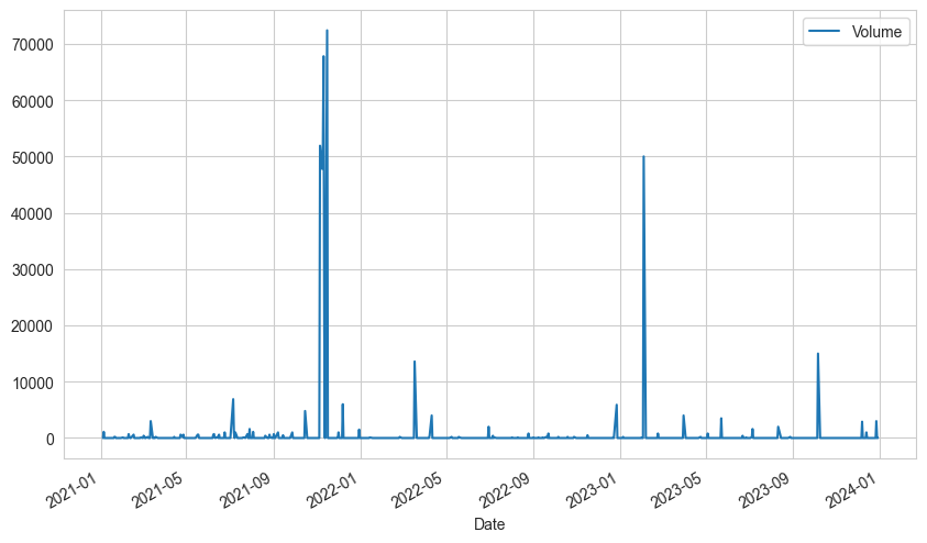
1
2
| smg_data['Volume'].plot(legend=True,figsize=(10,6))
#historical view of volume for San Miguel Corp
|
<Axes: xlabel='Date'>
Pivot a table from datetime
1
2
3
4
5
6
7
| plt.figure(figsize=(10, 6))
sns.lineplot(x='Date', y='Volume', data=jbf_data, marker='o')
plt.xticks(rotation=45)
plt.title('Jollibee Foods Corps')
plt.xlabel('Volume over Year and Month')
plt.tight_layout()
plt.show()
|
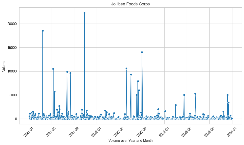
historical view of volume for Jollibee
| Close | High | Low | Open | Volume |
|---|
| Date | | | | | |
|---|
| 2021-01-04 | 2.765748 | 2.765748 | 2.765748 | 2.765748 | 0 |
|---|
| 2021-01-05 | 2.765748 | 2.765748 | 2.765748 | 2.765748 | 0 |
|---|
| 2021-01-06 | 2.765748 | 2.765748 | 2.765748 | 2.765748 | 0 |
|---|
| 2021-01-07 | 2.765748 | 2.765748 | 2.765748 | 2.765748 | 0 |
|---|
| 2021-01-08 | 2.844769 | 2.844769 | 2.844769 | 2.844769 | 5000 |
|---|
| ... | ... | ... | ... | ... | ... |
|---|
| 2023-12-22 | 1.870327 | 1.870327 | 1.870327 | 1.870327 | 0 |
|---|
| 2023-12-26 | 1.831961 | 1.831961 | 1.831961 | 1.831961 | 7600 |
|---|
| 2023-12-27 | 1.831961 | 1.831961 | 1.831961 | 1.831961 | 0 |
|---|
| 2023-12-28 | 1.831961 | 1.831961 | 1.831961 | 1.831961 | 0 |
|---|
| 2023-12-29 | 1.927875 | 1.927875 | 1.927875 | 1.927875 | 2500 |
|---|
753 rows × 5 columns
1
2
3
| # Convert 'date_column' to datetime format
uvr_data = uvr_data.reset_index(drop=False)
display(uvr_data)
|
| Date | Close | High | Low | Open | Volume |
|---|
| 0 | 2021-01-04 | 2.765748 | 2.765748 | 2.765748 | 2.765748 | 0 |
|---|
| 1 | 2021-01-05 | 2.765748 | 2.765748 | 2.765748 | 2.765748 | 0 |
|---|
| 2 | 2021-01-06 | 2.765748 | 2.765748 | 2.765748 | 2.765748 | 0 |
|---|
| 3 | 2021-01-07 | 2.765748 | 2.765748 | 2.765748 | 2.765748 | 0 |
|---|
| 4 | 2021-01-08 | 2.844769 | 2.844769 | 2.844769 | 2.844769 | 5000 |
|---|
| ... | ... | ... | ... | ... | ... | ... |
|---|
| 748 | 2023-12-22 | 1.870327 | 1.870327 | 1.870327 | 1.870327 | 0 |
|---|
| 749 | 2023-12-26 | 1.831961 | 1.831961 | 1.831961 | 1.831961 | 7600 |
|---|
| 750 | 2023-12-27 | 1.831961 | 1.831961 | 1.831961 | 1.831961 | 0 |
|---|
| 751 | 2023-12-28 | 1.831961 | 1.831961 | 1.831961 | 1.831961 | 0 |
|---|
| 752 | 2023-12-29 | 1.927875 | 1.927875 | 1.927875 | 1.927875 | 2500 |
|---|
753 rows × 6 columns
1
2
3
4
5
| sns.set_theme(rc={'figure.figsize':(11.7,8.27)})
sns.lineplot(data=smg_data, x='Date', y='Close', label='San Miguel')
sns.lineplot(data=delm_data, x='Date', y='Close', label='Mondelez')
sns.lineplot(data=uvr_data, x='Date', y='Close', label='Robina')
sns.lineplot(data=jbf_data, x='Date', y='Close', label='Jabee')
|
<Axes: xlabel='Date', ylabel='Close'>
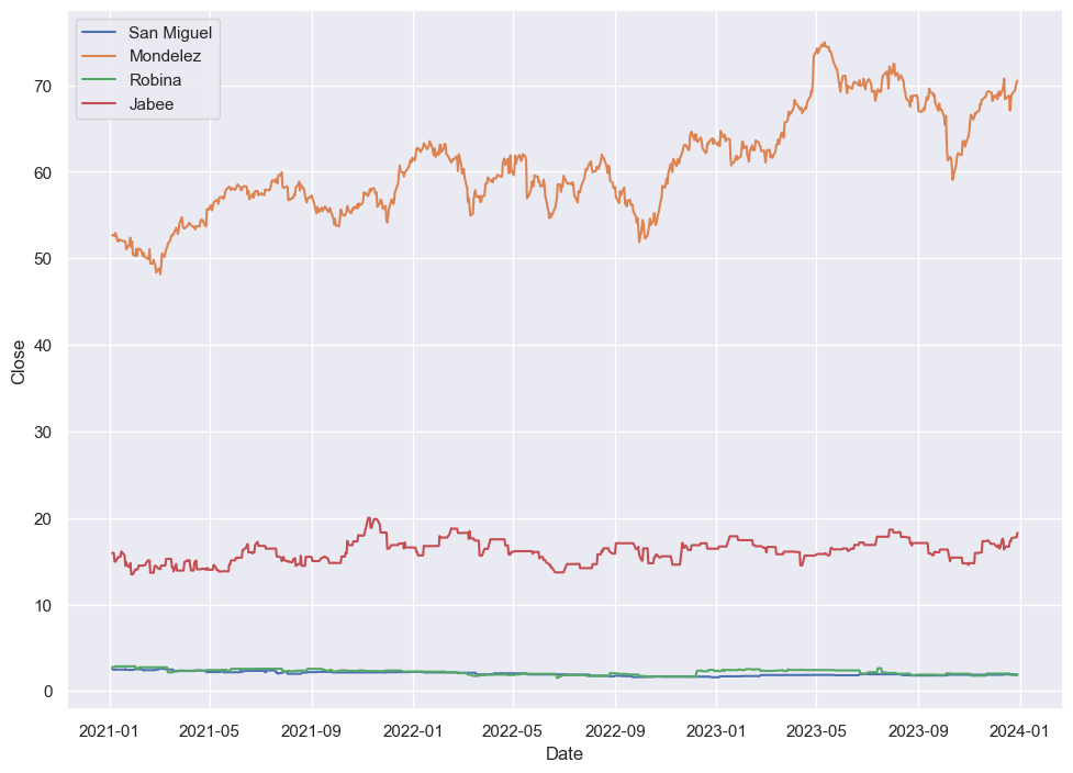
historical comparison of Closing price of Stocks
1
2
3
| smg_data = smg_data.reset_index(drop=False)
jbf_data = jbf_data.reset_index(drop=False)
delm_data = delm_data.reset_index(drop=False)
|
1
2
3
4
5
| smg_data.insert(0, 'Name', 'San Miguel Corp')
jbf_data.insert(0, 'Name', 'Jollibee Food Corp')
delm_data.insert(0, 'Name', 'Mondelez International')
uvr_data.insert(0, 'Name', 'Universal Robina Corp')
#adding a columns Name in the data frame
|
1
2
3
4
| # The comp stocks we'll use for this analysis
comp_list = [smg_data,jbf_data,uvr_data,delm_data]
#merging all the companies
comp_listGlobal = pd.concat(comp_list)
|
1
| display(comp_listGlobal)
|
| Name | Date | Close | High | Low | Open | Volume |
|---|
| 0 | San Miguel Corp | 2021-01-04 | 2.550820 | 2.550820 | 2.550820 | 2.550820 | 0 |
|---|
| 1 | San Miguel Corp | 2021-01-05 | 2.479167 | 2.479167 | 2.479167 | 2.479167 | 1100 |
|---|
| 2 | San Miguel Corp | 2021-01-06 | 2.479167 | 2.479167 | 2.479167 | 2.479167 | 0 |
|---|
| 3 | San Miguel Corp | 2021-01-07 | 2.479167 | 2.479167 | 2.479167 | 2.479167 | 0 |
|---|
| 4 | San Miguel Corp | 2021-01-08 | 2.479167 | 2.479167 | 2.479167 | 2.479167 | 0 |
|---|
| ... | ... | ... | ... | ... | ... | ... | ... |
|---|
| 748 | Mondelez International | 2023-12-22 | 68.921280 | 69.269710 | 68.476065 | 68.553496 | 4109000 |
|---|
| 749 | Mondelez International | 2023-12-26 | 69.405212 | 69.589108 | 68.718033 | 68.911602 | 4002900 |
|---|
| 750 | Mondelez International | 2023-12-27 | 69.889145 | 69.937541 | 69.240681 | 69.463284 | 4061500 |
|---|
| 751 | Mondelez International | 2023-12-28 | 70.351608 | 70.439228 | 69.796662 | 69.884282 | 4095300 |
|---|
| 752 | Mondelez International | 2023-12-29 | 70.517113 | 70.731304 | 70.205564 | 70.234771 | 4658600 |
|---|
3012 rows × 7 columns
1
| sns.lineplot(data=comp_listGlobal,x="Date", y="Close", hue="Name", style="Name")
|
<Axes: xlabel='Date', ylabel='Close'>
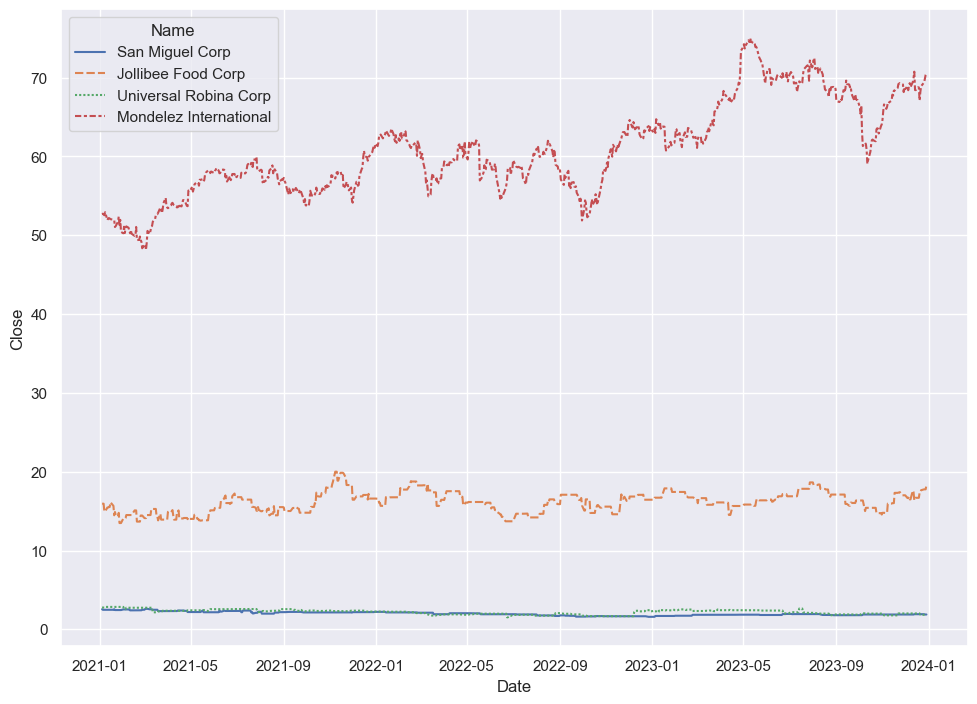
This is a much simple code of historical comparison of Closing price of Stocks
1
2
3
| #pivot a new data frame here
CloseDF = comp_listGlobal.pivot(index='Date', columns='Name', values=['Close'])
display(CloseDF)
|
| Close |
|---|
| Name | Jollibee Food Corp | Mondelez International | San Miguel Corp | Universal Robina Corp |
|---|
| Date | | | | |
|---|
| 2021-01-04 | 15.941961 | 52.686432 | 2.550820 | 2.765748 |
|---|
| 2021-01-05 | 15.941961 | 52.741009 | 2.479167 | 2.765748 |
|---|
| 2021-01-06 | 15.941961 | 52.640957 | 2.479167 | 2.765748 |
|---|
| 2021-01-07 | 14.946193 | 52.540890 | 2.479167 | 2.765748 |
|---|
| 2021-01-08 | 14.946193 | 52.932041 | 2.479167 | 2.844769 |
|---|
| ... | ... | ... | ... | ... |
|---|
| 2023-12-22 | 17.654762 | 68.921280 | 1.920405 | 1.870327 |
|---|
| 2023-12-26 | 17.764172 | 69.405212 | 1.920405 | 1.831961 |
|---|
| 2023-12-27 | 17.764172 | 69.889145 | 1.880809 | 1.831961 |
|---|
| 2023-12-28 | 17.764172 | 70.351608 | 1.880809 | 1.831961 |
|---|
| 2023-12-29 | 18.291327 | 70.517113 | 1.880809 | 1.927875 |
|---|
753 rows × 4 columns
1
2
| # Calculate the daily return percent of all stocks and store them
comp_returns = CloseDF.pct_change()
|
| Close |
|---|
| Name | Jollibee Food Corp | Mondelez International | San Miguel Corp | Universal Robina Corp |
|---|
| Date | | | | |
|---|
| 2021-01-04 | NaN | NaN | NaN | NaN |
|---|
| 2021-01-05 | 0.000000 | 0.001036 | -0.028090 | 0.000000 |
|---|
| 2021-01-06 | 0.000000 | -0.001897 | 0.000000 | 0.000000 |
|---|
| 2021-01-07 | -0.062462 | -0.001901 | 0.000000 | 0.000000 |
|---|
| 2021-01-08 | 0.000000 | 0.007445 | 0.000000 | 0.028571 |
|---|
| ... | ... | ... | ... | ... |
|---|
| 2023-12-22 | 0.018944 | 0.010644 | 0.000000 | 0.000000 |
|---|
| 2023-12-26 | 0.006197 | 0.007022 | 0.000000 | -0.020513 |
|---|
| 2023-12-27 | 0.000000 | 0.006973 | -0.020619 | 0.000000 |
|---|
| 2023-12-28 | 0.000000 | 0.006617 | 0.000000 | 0.000000 |
|---|
| 2023-12-29 | 0.029675 | 0.002353 | 0.000000 | 0.052356 |
|---|
753 rows × 4 columns
1
2
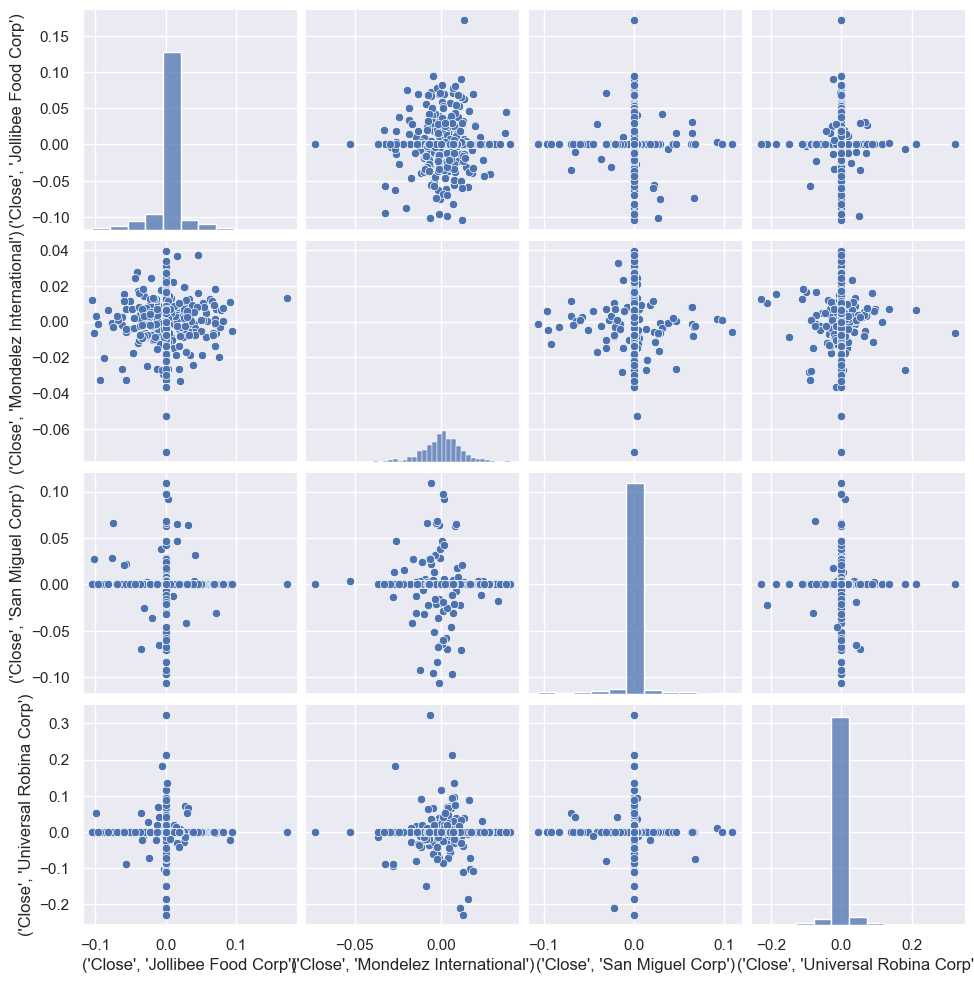
| sns.pairplot(comp_returns.dropna())
#correlation analysis for all possible pairs of stocks in our food stock ticker list.
|
<seaborn.axisgrid.PairGrid at 0x1e5652c4500>
1
2
3
4
5
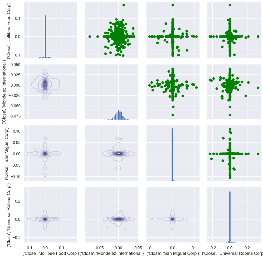
| # Mixed plot to visualize the correlation between all food stocks
comp_fig = sns.PairGrid(comp_returns.dropna())
comp_fig.map_upper(plt.scatter,color='green')
comp_fig.map_lower(sns.kdeplot,cmap='Purples_d')
comp_fig.map_diag(plt.hist,bins=30)
|
<seaborn.axisgrid.PairGrid at 0x1e56934adb0>
1
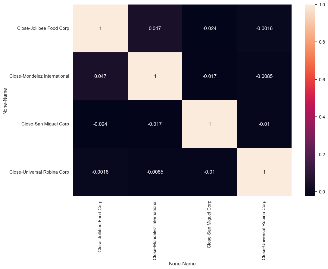
2
3
| # Correlation plot for the daily returns of all stocks
comp_returns_corr= comp_returns.dropna().corr()
sns.heatmap(comp_returns_corr,annot=True)
|
<Axes: xlabel='None-Name', ylabel='None-Name'>