Before Getting Started make sure you got pip and python 3.8 or higher
I am using a Jupyter Notebook and I might already have these libraries but going to run it just in case
pip install pandas numpy matplotlib yfinance seabornThese are the following companies we are going to use for analyzing: San Miguel Corporation (SMGBF) Jollibee Foods Corporation (JBFCY) Universal Robina Corporation (UVRBF) Mondelez International, Inc.(MDLZ)
yfinance is a library for fetching historical stock data
pandas for Data Exploration and Data Cleaning
seaborn and matplotlib for Data Visualization (Honestly when I heard about these in 2016 or 17 I thought these were YouTubers)
#pandas and NumPy imports
import pandas as pd
from pandas import Series,DataFrame
import numpy as np
# For Visualization
import matplotlib.pyplot as plt
import seaborn as sns
sns.set_style('whitegrid')
%matplotlib inlineimport os #for files read/write
from datetime import datetime # For time stamps
import yfinance as yf #fetching the data stock
from __future__ import division# For division in Python 3# Fetch stock data
def fetch_stock_data(ticker, start_date, end_date):
stock_data = yf.download(ticker, start=start_date, end=end_date)
return stock_data
smg_data = fetch_stock_data('SMGBF', '2021-01-01', '2023-12-31')
jbf_data = fetch_stock_data('JBFCY', '2021-01-01', '2023-12-31')
uvr_data = fetch_stock_data('UVRBF', '2021-01-01', '2023-12-31')
delm_data = fetch_stock_data('MDLZ', '2021-01-01', '2023-12-31')[*********************100%***********************] 1 of 1 completed
[*********************100%***********************] 1 of 1 completed
[*********************100%***********************] 1 of 1 completed
[*********************100%***********************] 1 of 1 completed
checking data
print(smg_data.head())
print(jbf_data.head())
print(uvr_data.head())
print(delm_data.head())
Price Close High Low Open Volume
Ticker SMGBF SMGBF SMGBF SMGBF SMGBF
Date
2021-01-04 2.550820 2.550820 2.550820 2.550820 0
2021-01-05 2.479167 2.479167 2.479167 2.479167 1100
2021-01-06 2.479167 2.479167 2.479167 2.479167 0
2021-01-07 2.479167 2.479167 2.479167 2.479167 0
2021-01-08 2.479167 2.479167 2.479167 2.479167 0
Price Close High Low Open Volume
Ticker JBFCY JBFCY JBFCY JBFCY JBFCY
Date
2021-01-04 15.941961 15.941961 15.941961 15.941961 500
2021-01-05 15.941961 15.941961 15.941961 15.941961 0
2021-01-06 15.941961 15.941961 15.941961 15.941961 0
2021-01-07 14.946193 15.139546 14.946193 14.946193 1100
2021-01-08 14.946193 14.946193 14.946193 14.946193 0
Price Close High Low Open Volume
Ticker UVRBF UVRBF UVRBF UVRBF UVRBF
Date
2021-01-04 2.765748 2.765748 2.765748 2.765748 0
2021-01-05 2.765748 2.765748 2.765748 2.765748 0
2021-01-06 2.765748 2.765748 2.765748 2.765748 0
2021-01-07 2.765748 2.765748 2.765748 2.765748 0
2021-01-08 2.844769 2.844769 2.844769 2.844769 5000
Price Close High Low Open Volume
Ticker MDLZ MDLZ MDLZ MDLZ MDLZ
Date
2021-01-04 52.686432 54.578488 52.149747 53.204931 9187200
2021-01-05 52.741009 52.868358 52.140646 52.659141 5421900
2021-01-06 52.640957 53.059395 52.449933 52.750116 7663200
2021-01-07 52.540890 53.077578 52.167937 52.504507 8589100
2021-01-08 52.932041 53.004814 52.149752 52.186135 6642700
checking for dupes
print(smg_data.isnull().sum())
print(jbf_data.isnull().sum())
print(uvr_data.isnull().sum())
print(delm_data.isnull().sum())type(smg_data) #I just like to check what type of data we are working withchecking excel file
path = 'fnbStocks.xlsx'
isExist = os.path.exists(path)
print(isExist)
True
So there was an error making the excel and here you would see that the columns for our data frame has two values
display(smg_data)| Price | Close | High | Low | Open | Volume |
|---|---|---|---|---|---|
| Ticker | SMGBF | SMGBF | SMGBF | SMGBF | SMGBF |
| Date | |||||
| 2021-01-04 | 2.550820 | 2.550820 | 2.550820 | 2.550820 | 0 |
| 2021-01-05 | 2.479167 | 2.479167 | 2.479167 | 2.479167 | 1100 |
| 2021-01-06 | 2.479167 | 2.479167 | 2.479167 | 2.479167 | 0 |
| 2021-01-07 | 2.479167 | 2.479167 | 2.479167 | 2.479167 | 0 |
| 2021-01-08 | 2.479167 | 2.479167 | 2.479167 | 2.479167 | 0 |
| ... | ... | ... | ... | ... | ... |
| 2023-12-22 | 1.920405 | 1.920405 | 1.920405 | 1.920405 | 0 |
| 2023-12-26 | 1.920405 | 1.920405 | 1.920405 | 1.920405 | 0 |
| 2023-12-27 | 1.880809 | 1.969900 | 1.880809 | 1.969900 | 3000 |
| 2023-12-28 | 1.880809 | 1.880809 | 1.880809 | 1.880809 | 0 |
| 2023-12-29 | 1.880809 | 1.880809 | 1.880809 | 1.880809 | 0 |
753 rows × 5 columns
display(smg_data.columns)MultiIndex([( 'Close', 'SMGBF'),
( 'High', 'SMGBF'),
( 'Low', 'SMGBF'),
( 'Open', 'SMGBF'),
('Volume', 'SMGBF')],
names=['Price', 'Ticker'])
reassigned every dataframe with a new column
smg_data.columns= [col[0] for col in smg_data.columns]
jbf_data.columns=[col[0] for col in jbf_data.columns]
uvr_data.columns=[col[0] for col in uvr_data.columns]
delm_data.columns=[col[0] for col in delm_data.columns]display(smg_data.columns)Index(['Close', 'High', 'Low', 'Open', 'Volume'], dtype='object')
display(smg_data)| Close | High | Low | Open | Volume | |
|---|---|---|---|---|---|
| Date | |||||
| 2021-01-04 | 2.550820 | 2.550820 | 2.550820 | 2.550820 | 0 |
| 2021-01-05 | 2.479167 | 2.479167 | 2.479167 | 2.479167 | 1100 |
| 2021-01-06 | 2.479167 | 2.479167 | 2.479167 | 2.479167 | 0 |
| 2021-01-07 | 2.479167 | 2.479167 | 2.479167 | 2.479167 | 0 |
| 2021-01-08 | 2.479167 | 2.479167 | 2.479167 | 2.479167 | 0 |
| ... | ... | ... | ... | ... | ... |
| 2023-12-22 | 1.920405 | 1.920405 | 1.920405 | 1.920405 | 0 |
| 2023-12-26 | 1.920405 | 1.920405 | 1.920405 | 1.920405 | 0 |
| 2023-12-27 | 1.880809 | 1.969900 | 1.880809 | 1.969900 | 3000 |
| 2023-12-28 | 1.880809 | 1.880809 | 1.880809 | 1.880809 | 0 |
| 2023-12-29 | 1.880809 | 1.880809 | 1.880809 | 1.880809 | 0 |
753 rows × 5 columns
with pd.ExcelWriter('fnbStocks.xlsx') as writer:
    smg_data.to_excel(writer, sheet_name='SanMiguel')
    jbf_data.to_excel(writer, sheet_name='Jollibee')
    uvr_data.to_excel(writer, sheet_name='Robina')
    delm_data.to_excel(writer, sheet_name='DelMonte')
check to see if your excel file is good.
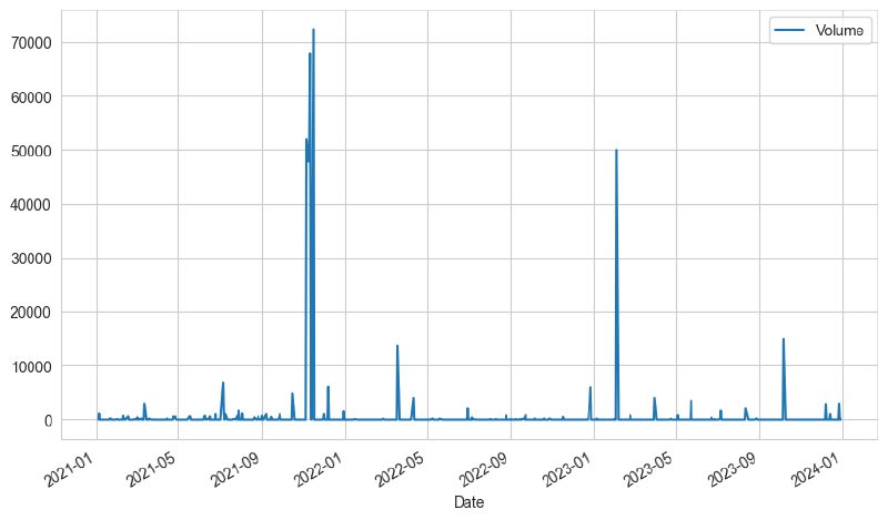
smg_data['Volume'].plot(legend=True,figsize=(10,6))
#historical view of volume for San Miguel Corp
<Axes: xlabel='Date'>
Pivot a table from datetime
plt.figure(figsize=(10, 6))
sns.lineplot(x='Date', y='Volume', data=jbf_data, marker='o')
plt.xticks(rotation=45)
plt.title('Jollibee Foods Corps')
plt.xlabel('Volume over Year and Month')
plt.tight_layout()
plt.show()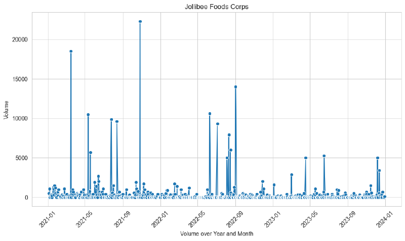
historical view of volume for Jollibee
display(uvr_data)| Close | High | Low | Open | Volume | |
|---|---|---|---|---|---|
| Date | |||||
| 2021-01-04 | 2.765748 | 2.765748 | 2.765748 | 2.765748 | 0 |
| 2021-01-05 | 2.765748 | 2.765748 | 2.765748 | 2.765748 | 0 |
| 2021-01-06 | 2.765748 | 2.765748 | 2.765748 | 2.765748 | 0 |
| 2021-01-07 | 2.765748 | 2.765748 | 2.765748 | 2.765748 | 0 |
| 2021-01-08 | 2.844769 | 2.844769 | 2.844769 | 2.844769 | 5000 |
| ... | ... | ... | ... | ... | ... |
| 2023-12-22 | 1.870327 | 1.870327 | 1.870327 | 1.870327 | 0 |
| 2023-12-26 | 1.831961 | 1.831961 | 1.831961 | 1.831961 | 7600 |
| 2023-12-27 | 1.831961 | 1.831961 | 1.831961 | 1.831961 | 0 |
| 2023-12-28 | 1.831961 | 1.831961 | 1.831961 | 1.831961 | 0 |
| 2023-12-29 | 1.927875 | 1.927875 | 1.927875 | 1.927875 | 2500 |
753 rows × 5 columns
# Convert 'date_column' to datetime format
uvr_data = uvr_data.reset_index(drop=False)
display(uvr_data)| Date | Close | High | Low | Open | Volume | |
|---|---|---|---|---|---|---|
| 0 | 2021-01-04 | 2.765748 | 2.765748 | 2.765748 | 2.765748 | 0 |
| 1 | 2021-01-05 | 2.765748 | 2.765748 | 2.765748 | 2.765748 | 0 |
| 2 | 2021-01-06 | 2.765748 | 2.765748 | 2.765748 | 2.765748 | 0 |
| 3 | 2021-01-07 | 2.765748 | 2.765748 | 2.765748 | 2.765748 | 0 |
| 4 | 2021-01-08 | 2.844769 | 2.844769 | 2.844769 | 2.844769 | 5000 |
| ... | ... | ... | ... | ... | ... | ... |
| 748 | 2023-12-22 | 1.870327 | 1.870327 | 1.870327 | 1.870327 | 0 |
| 749 | 2023-12-26 | 1.831961 | 1.831961 | 1.831961 | 1.831961 | 7600 |
| 750 | 2023-12-27 | 1.831961 | 1.831961 | 1.831961 | 1.831961 | 0 |
| 751 | 2023-12-28 | 1.831961 | 1.831961 | 1.831961 | 1.831961 | 0 |
| 752 | 2023-12-29 | 1.927875 | 1.927875 | 1.927875 | 1.927875 | 2500 |
753 rows × 6 columns
sns.set_theme(rc={'figure.figsize':(11.7,8.27)})
sns.lineplot(data=smg_data, x='Date', y='Close', label='San Miguel')
sns.lineplot(data=delm_data, x='Date', y='Close', label='Mondelez')
sns.lineplot(data=uvr_data, x='Date', y='Close', label='Robina')
sns.lineplot(data=jbf_data, x='Date', y='Close', label='Jabee')
<Axes: xlabel='Date', ylabel='Close'>
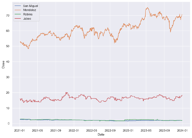
historical comparison of Closing price of Stocks
smg_data = smg_data.reset_index(drop=False)
jbf_data = jbf_data.reset_index(drop=False)
delm_data = delm_data.reset_index(drop=False)smg_data.insert(0, 'Name', 'San Miguel Corp')
jbf_data.insert(0, 'Name', 'Jollibee Food Corp')
delm_data.insert(0, 'Name', 'Mondelez International')
uvr_data.insert(0, 'Name', 'Universal Robina Corp')
#adding a columns Name in the data frame# The comp stocks we'll use for this analysis
comp_list = [smg_data,jbf_data,uvr_data,delm_data]
#merging all the companies
comp_listGlobal = pd.concat(comp_list)display(comp_listGlobal)| Name | Date | Close | High | Low | Open | Volume | |
|---|---|---|---|---|---|---|---|
| 0 | San Miguel Corp | 2021-01-04 | 2.550820 | 2.550820 | 2.550820 | 2.550820 | 0 |
| 1 | San Miguel Corp | 2021-01-05 | 2.479167 | 2.479167 | 2.479167 | 2.479167 | 1100 |
| 2 | San Miguel Corp | 2021-01-06 | 2.479167 | 2.479167 | 2.479167 | 2.479167 | 0 |
| 3 | San Miguel Corp | 2021-01-07 | 2.479167 | 2.479167 | 2.479167 | 2.479167 | 0 |
| 4 | San Miguel Corp | 2021-01-08 | 2.479167 | 2.479167 | 2.479167 | 2.479167 | 0 |
| ... | ... | ... | ... | ... | ... | ... | ... |
| 748 | Mondelez International | 2023-12-22 | 68.921280 | 69.269710 | 68.476065 | 68.553496 | 4109000 |
| 749 | Mondelez International | 2023-12-26 | 69.405212 | 69.589108 | 68.718033 | 68.911602 | 4002900 |
| 750 | Mondelez International | 2023-12-27 | 69.889145 | 69.937541 | 69.240681 | 69.463284 | 4061500 |
| 751 | Mondelez International | 2023-12-28 | 70.351608 | 70.439228 | 69.796662 | 69.884282 | 4095300 |
| 752 | Mondelez International | 2023-12-29 | 70.517113 | 70.731304 | 70.205564 | 70.234771 | 4658600 |
3012 rows × 7 columns
sns.lineplot(data=comp_listGlobal,x="Date", y="Close", hue="Name", style="Name")<Axes: xlabel='Date', ylabel='Close'>
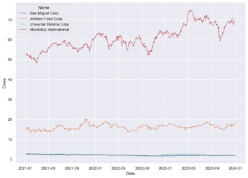
This is a much simple code of historical comparison of Closing price of Stocks
#pivot a new data frame here
CloseDF = comp_listGlobal.pivot(index='Date', columns='Name', values=['Close'])
display(CloseDF)| Close | ||||
|---|---|---|---|---|
| Name | Jollibee Food Corp | Mondelez International | San Miguel Corp | Universal Robina Corp |
| Date | ||||
| 2021-01-04 | 15.941961 | 52.686432 | 2.550820 | 2.765748 |
| 2021-01-05 | 15.941961 | 52.741009 | 2.479167 | 2.765748 |
| 2021-01-06 | 15.941961 | 52.640957 | 2.479167 | 2.765748 |
| 2021-01-07 | 14.946193 | 52.540890 | 2.479167 | 2.765748 |
| 2021-01-08 | 14.946193 | 52.932041 | 2.479167 | 2.844769 |
| ... | ... | ... | ... | ... |
| 2023-12-22 | 17.654762 | 68.921280 | 1.920405 | 1.870327 |
| 2023-12-26 | 17.764172 | 69.405212 | 1.920405 | 1.831961 |
| 2023-12-27 | 17.764172 | 69.889145 | 1.880809 | 1.831961 |
| 2023-12-28 | 17.764172 | 70.351608 | 1.880809 | 1.831961 |
| 2023-12-29 | 18.291327 | 70.517113 | 1.880809 | 1.927875 |
753 rows × 4 columns
# Calculate the daily return percent of all stocks and store them
comp_returns = CloseDF.pct_change()display(comp_returns)| Close | ||||
|---|---|---|---|---|
| Name | Jollibee Food Corp | Mondelez International | San Miguel Corp | Universal Robina Corp |
| Date | ||||
| 2021-01-04 | NaN | NaN | NaN | NaN |
| 2021-01-05 | 0.000000 | 0.001036 | -0.028090 | 0.000000 |
| 2021-01-06 | 0.000000 | -0.001897 | 0.000000 | 0.000000 |
| 2021-01-07 | -0.062462 | -0.001901 | 0.000000 | 0.000000 |
| 2021-01-08 | 0.000000 | 0.007445 | 0.000000 | 0.028571 |
| ... | ... | ... | ... | ... |
| 2023-12-22 | 0.018944 | 0.010644 | 0.000000 | 0.000000 |
| 2023-12-26 | 0.006197 | 0.007022 | 0.000000 | -0.020513 |
| 2023-12-27 | 0.000000 | 0.006973 | -0.020619 | 0.000000 |
| 2023-12-28 | 0.000000 | 0.006617 | 0.000000 | 0.000000 |
| 2023-12-29 | 0.029675 | 0.002353 | 0.000000 | 0.052356 |
753 rows × 4 columns
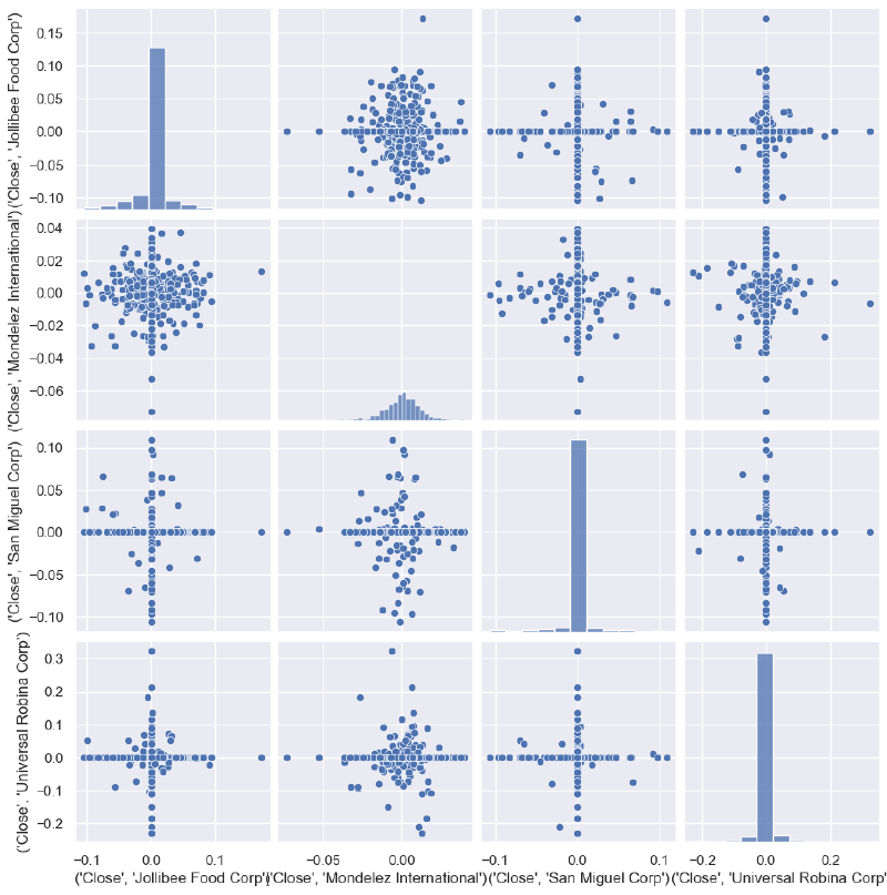
sns.pairplot(comp_returns.dropna())
#correlation analysis for all possible pairs of stocks in our food stock ticker list.
<seaborn.axisgrid.PairGrid at 0x1e5652c4500>
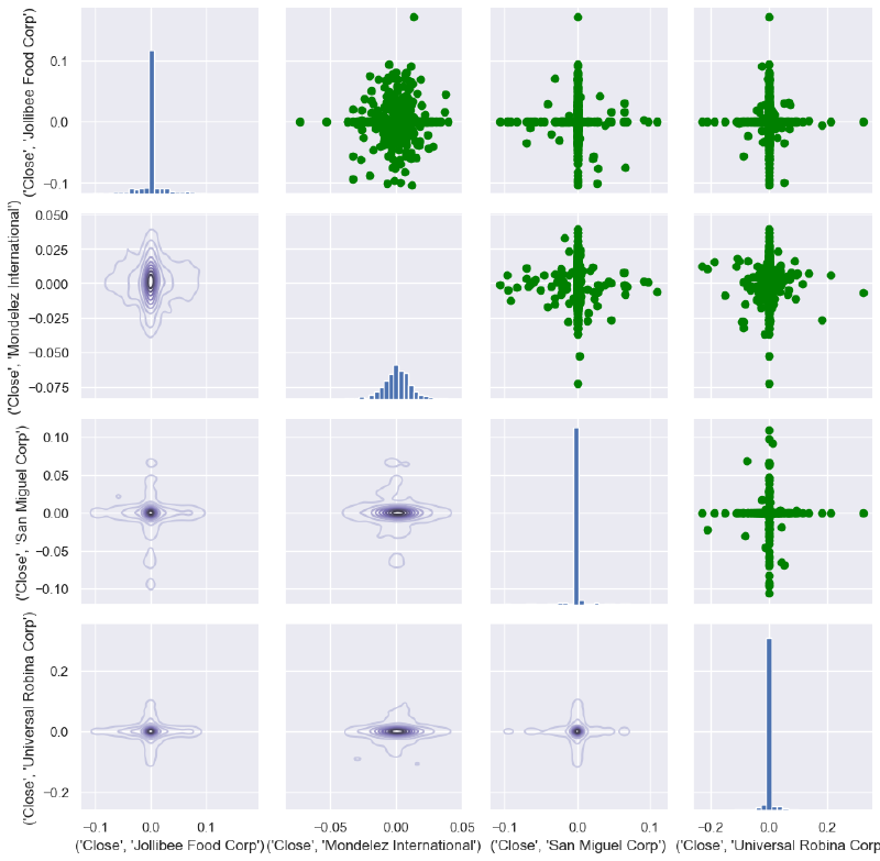
# Mixed plot to visualize the correlation between all food stocks
comp_fig = sns.PairGrid(comp_returns.dropna())
comp_fig.map_upper(plt.scatter,color='green')
comp_fig.map_lower(sns.kdeplot,cmap='Purples_d')
comp_fig.map_diag(plt.hist,bins=30)
<seaborn.axisgrid.PairGrid at 0x1e56934adb0>
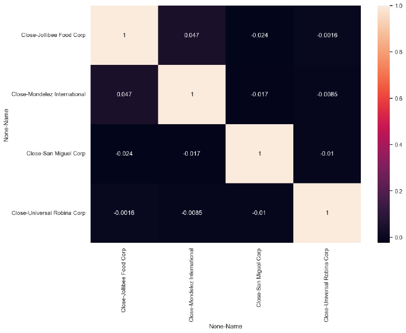
# Correlation plot for the daily returns of all stocks
comp_returns_corr= comp_returns.dropna().corr()
sns.heatmap(comp_returns_corr,annot=True)
<Axes: xlabel='None-Name', ylabel='None-Name'>